Poverty and Inequality Platform (PIP):
An introduction using R and Stata

Diana C. Garcia Rojas

August 2026

Outline

Introduction to the Poverty and Inequality Platform (PIP)
PIP user interface
Accessing the PIP API with R and Stata
Exercises
Additional resources

1. Introduction

Poverty data at the World Bank

The World Bank mission is to end extreme poverty and boost shared prosperity on a livable planet.
To that end, the World Bank often helps countries field household surveys to track welfare.
Some countries do not receive assistance yet the Bank is granted access to the data through collaborations with the National Statistical Office.
For high-income countries, poverty data is sourced from the Luxembourg Income Study or EU-SILC.

The Poverty and Inequality Platform (PIP)

PIP is the source of poverty and inequality data for the World Bank.
PIP is the source of data for several targets of the Sustainable Development Goals on ending poverty (SDG1) and reducing inequality (SDG10).
PIP is the joint collaboration between different parts of the World Bank through the Global Poverty Working Group
- Development Data Group
- Development Research Group
- Poverty and Equity Global Department

PIP motivation

Scope: PIP is the World Bank’s data portal for poverty, prosperity, and inequality estimates.
Accessibility: PIP data is available through Application Programming Interface (API)
- User Interface (UI) – for quick data access and visualizations
- Stata and R wrappers – for advanced users, researchers, students
- Microdata access (for some surveys) through Microdata Online.
Open data, open code, reproducible research:
- PIP code is publicly available, and the PIP Methodology Handbook provides details on the poverty, prosperity, and inequality estimates reported in PIP.
- PIP typically is updated twice a year - Spring/Fall. One can, however, access various vintages of the data.

PIP: Transparency

All code necessary to create the poverty estimates are publicly available (https://github.com/PIP-Technical-Team)

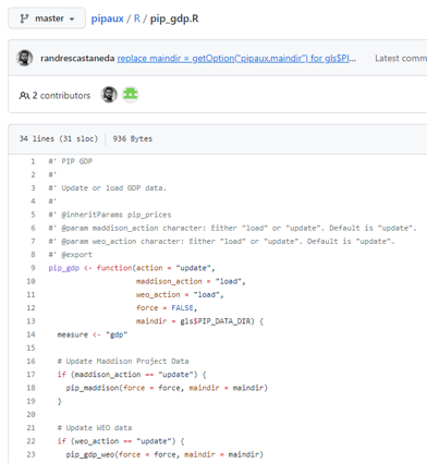
PIP: Transparency

A description of the entire methodology is available in a technical handbook (https://datanalytics.worldbank.org/PIP-Methodology/)

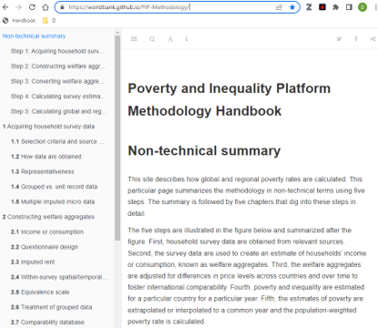
Data release notes and other publications

Publications are available detailing the updates in each release, methodological assumptions, and other technical improvements (https://pip.worldbank.org/publication/)

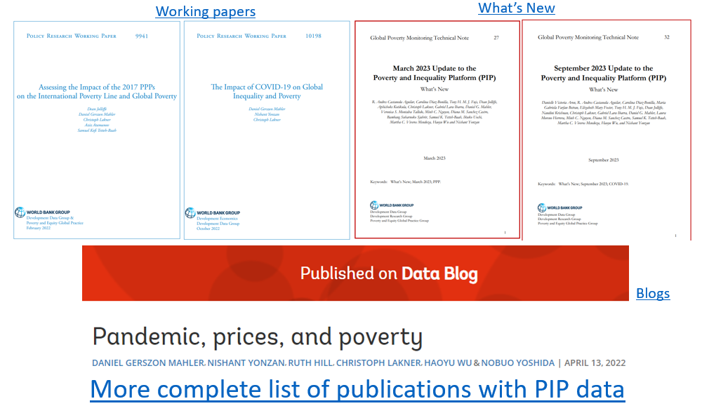
Data on inequality

For each survey, PIP output reports inequality and shared prosperity measures like the Gini, MLD, polarization index, the decile share of income or consumption, and the Prosperity Gap.
In addition, PIP has a dedicated dashboard that visualize inequality trends and changes. This is available through the Further Data & Indicators page in PIP UI.
We also report the average and threshold income of each percentile for each survey. THis is also available through the Further Data & Indicators page in the PIP website.

Acquiring Household Data

Sources:
- LIC: Surveys collected by National Statistical Offices
- HIC:
  - Europe: EU-SILC
  - Other (and earlier years): Luxembourg Income Study (LIS)
Data input type: welfare (consumption/income) data at the household or group level

Constructing Welfare Aggregates

Income vs Consumption (welfare_type) -> consumption preferred.
Bottom coding
Micro or Grouped Data (distribution_type)
Additional comparability considerations:
- Questionnaire design changes
- Equivalence scales (->not used)
- Spatio/temporal adjustments
- Tracked in PIP: comparable_spell and survey_comparability.

Adjusting Welfare Aggregates

Consumer Price Indices (CPIs) & Purchasing Power Parities (PPPs)
Derivation of the International Poverty Line (poverty_line)
- $3.00/day in 2021 PPP -> based on the median of harmonized national poverty lines from poorest countries
Derivation of higher poverty lines
- $4.20 and $8.30 in 2021 PPP -> based on median values of national poverty lines of lower- and upper-middle income countries, respectively.
Derivation of societal poverty line (spl) -> varies across countries in accord with the average estimated cost of meeting basic needs.

Calculating survey estimates

Poverty and Inequality metrics are calculated using adjusted welfare aggregates.
All methodology is available in the PIP Methodological Handbook on the website.
Source code is available on github through the package wbpip.

Calculating regional aggregates

Extrapolations and/or Interpolations (fill_gaps)
Nowcasts (nowcast)
Regional classification
Population adjustments
Coverage rules applied

2. Accessing PIP through the user interface

3. Accessing PIP in R and Stata

Installation

R
Stata

# To install the pipr package, you first need to install the devtools package
install.packages("devtools")
# The devtools package allows you to install pipr through GitHub
devtools::install_github("worldbank/pipr")
# Now load pipr
library(pipr)
# I'll use dplyr a lot in these slides, so best to load it as well
library(dplyr)

More information: https://worldbank.github.io/pipr/

* First install github, which lets you install Stata packages from GitHub
net install github, from("https://haghish.github.io/github/")
* Now install the pip package
github install worldbank/pip

More information: https://github.com/worldbank/pip/

Two main functions

R
Stata

get_stats(): country estimates of poverty and inequality
- each row identifies a unique combination of country_code, year, reporting_level, and welfare_type
- reporting_level: Mostly national, but can be urban or rural
- welfare_type: Income or consumption
get_wb(): regional/global estimates of poverty and inequality
- each row identifies a unique combination of region_code and year.

pip cl: country estimates of poverty and inequality
- each row identifies a unique combination of country_code, year, reporting_level, and welfare_type
- reporting_level: Mostly national, but can be urban or rural
- welfare_type: Income or consumption
pip wb: regional/global estimates of poverty and inequality
- each row identifies a unique combination of region_code and year.

Country-level estimates

R code
R output
Stata code
Stata output

get_stats()

# A tibble: 2,584 × 44
   region_name       region_code country_name country_code  year reporting_level
   <chr>             <chr>       <chr>        <chr>        <dbl> <chr>          
 1 Sub-Saharan Afri… SSF         Angola       AGO           2000 national       
 2 Sub-Saharan Afri… SSF         Angola       AGO           2008 national       
 3 Sub-Saharan Afri… SSF         Angola       AGO           2018 national       
 4 Europe & Central… ECS         Albania      ALB           1996 national       
 5 Europe & Central… ECS         Albania      ALB           2002 national       
 6 Europe & Central… ECS         Albania      ALB           2005 national       
 7 Europe & Central… ECS         Albania      ALB           2008 national       
 8 Europe & Central… ECS         Albania      ALB           2012 national       
 9 Europe & Central… ECS         Albania      ALB           2014 national       
10 Europe & Central… ECS         Albania      ALB           2015 national       
# ℹ 2,574 more rows
# ℹ 38 more variables: survey_acronym <chr>, survey_coverage <chr>,
#   welfare_time <dbl>, welfare_type <chr>, survey_comparability <dbl>,
#   comparable_spell <chr>, poverty_line <dbl>, headcount <dbl>,
#   poverty_gap <dbl>, poverty_severity <dbl>, watts <dbl>, mean <dbl>,
#   median <dbl>, mld <dbl>, gini <dbl>, polarization <dbl>, decile1 <dbl>,
#   decile2 <dbl>, decile3 <dbl>, decile4 <dbl>, decile5 <dbl>, …

pip cl, clear
list country_code year welfare_type reporting_level headcount gini in 1/5

version in use 20260324_2021_01_02_PROD

first observation

  +------------------------------------------------------------------------+
  | country_code   year   poverty_line   headcount     mean   welfare_type |
  |------------------------------------------------------------------------|
  |          AGO   2000           3.00      0.2695   8.3803    consumption |
  +------------------------------------------------------------------------+
Click here to display how to cite

     +--------------------------------------------------------------+
     | count~de   year   welfare_~pe   report~l   headco~t     gini |
     |--------------------------------------------------------------|
  1. |      AGO   2000   consumption   national     0.2695   0.5195 |
  2. |      AGO   2008   consumption   national     0.2208   0.4272 |
  3. |      AGO   2018   consumption   national     0.3929   0.5126 |
  4. |      ALB   1996   consumption   national     0.0297   0.2701 |
  5. |      ALB   2002   consumption   national     0.0419   0.3174 |
     +--------------------------------------------------------------+

Variables

R code
R output
Stata code
Stata output

glimpse(get_stats())

Rows: 2,584
Columns: 44
$ region_name          <chr> "Sub-Saharan Africa", "Sub-Saharan Africa", "Sub-…
$ region_code          <chr> "SSF", "SSF", "SSF", "ECS", "ECS", "ECS", "ECS", …
$ country_name         <chr> "Angola", "Angola", "Angola", "Albania", "Albania…
$ country_code         <chr> "AGO", "AGO", "AGO", "ALB", "ALB", "ALB", "ALB", …
$ year                 <dbl> 2000, 2008, 2018, 1996, 2002, 2005, 2008, 2012, 2…
$ reporting_level      <chr> "national", "national", "national", "national", "…
$ survey_acronym       <chr> "HBS", "IBEP-MICS", "IDREA", "EWS", "LSMS", "LSMS…
$ survey_coverage      <chr> "national", "national", "national", "national", "…
$ welfare_time         <dbl> 2000.21, 2008.50, 2018.17, 1996.00, 2002.00, 2005…
$ welfare_type         <chr> "consumption", "consumption", "consumption", "con…
$ survey_comparability <dbl> 0, 1, 2, 0, 1, 1, 1, 1, 2, 2, 2, 4, 2, 4, 3, 4, 3…
$ comparable_spell     <chr> "2000", "2008", "2018", "1996", "2002 - 2012", "2…
$ poverty_line         <dbl> 3, 3, 3, 3, 3, 3, 3, 3, 3, 3, 3, 3, 3, 3, 3, 3, 3…
$ headcount            <dbl> 0.269546383, 0.220795824, 0.392947051, 0.02967841…
$ poverty_gap          <dbl> 0.1191549532, 0.0666666645, 0.1629885084, 0.00439…
$ poverty_severity     <dbl> 7.064835e-02, 2.902800e-02, 8.930591e-02, 1.17603…
$ watts                <dbl> 0.1973895465, 0.0905210047, 0.2519774127, 0.00522…
$ mean                 <dbl> 8.380261, 7.401682, 6.218052, 8.442032, 8.628333,…
$ median               <dbl> 5.300380, 5.334158, 3.879510, 7.419330, 7.117154,…
$ mld                  <dbl> 0.5094919, 0.3116315, 0.4763749, 0.1191043, 0.164…
$ gini                 <dbl> 0.5194515, 0.4271551, 0.5126429, 0.2701034, 0.317…
$ polarization         <dbl> 0.4643389, 0.3913652, 0.4709815, 0.2412933, 0.268…
$ decile1              <dbl> 0.00990998, 0.02072270, 0.01334655, 0.03881788, 0…
$ decile2              <dbl> 0.02198698, 0.03356417, 0.02428161, 0.05279230, 0…
$ decile3              <dbl> 0.03341620, 0.04317617, 0.03332952, 0.06370657, 0…
$ decile4              <dbl> 0.04509489, 0.05302731, 0.04343721, 0.07524026, 0…
$ decile5              <dbl> 0.05646606, 0.06542599, 0.05582912, 0.08346224, 0…
$ decile6              <dbl> 0.07048204, 0.07923758, 0.06980908, 0.09245731, 0…
$ decile7              <dbl> 0.08817254, 0.09651189, 0.08869304, 0.10778961, 0…
$ decile8              <dbl> 0.1133977, 0.1229761, 0.1156761, 0.1261162, 0.119…
$ decile9              <dbl> 0.1593917, 0.1623416, 0.1593804, 0.1525077, 0.149…
$ decile10             <dbl> 0.4016820, 0.3230165, 0.3962174, 0.2071100, 0.253…
$ cpi                  <dbl> 0.006580985, 0.140636450, 0.571606031, 0.37247663…
$ ppp                  <dbl> 203.688736, 203.688736, 203.688736, 50.772305, 50…
$ pop                  <dbl> 16310860, 21996714, 31480496, 3168033, 3051010, 3…
$ gdp                  <dbl> 2172.463, 3559.195, 3196.790, 1683.770, 2297.109,…
$ hfce                 <dbl> NA, 1748.428, 2261.456, 1522.872, 1572.295, 1969.…
$ is_interpolated      <lgl> FALSE, FALSE, FALSE, FALSE, FALSE, FALSE, FALSE, …
$ distribution_type    <chr> "micro", "micro", "micro", "micro", "micro", "mic…
$ estimation_type      <chr> "survey", "survey", "survey", "survey", "survey",…
$ spl                  <dbl> 3.950, 3.967, 3.240, 5.010, 4.859, 5.450, 5.770, …
$ spr                  <dbl> 0.3714692, 0.3533580, 0.4216190, 0.2039019, 0.224…
$ pg                   <dbl> 9.6092024, 6.8387556, 10.9642421, 4.2094284, 4.42…
$ estimate_type        <chr> NA, NA, NA, NA, NA, NA, NA, NA, NA, NA, NA, NA, N…

describe

Contains data from C:\Users\wb535623\AppData\Local\Temp\ST_3074_000001.tmp
 Observations:         2,584                  WB poverty at country level (31 Aug 2026)
    Variables:            43                  31 Aug 2026 20:49
                                              (_dta has notes)
--------------------------------------------------------------------------------------------------------------------------------------------------------------------------------------------------------
Variable      Storage   Display    Value
    name         type    format    label      Variable label
--------------------------------------------------------------------------------------------------------------------------------------------------------------------------------------------------------
country_code    str3    %9s                   country/economy code
country_name    str30   %30s                  country/economy name
region_code     str3    %9s                   region code
region_name     str49   %49s                  region name
reporting_level str8    %9s                   reporting data level
year            int     %8.0g                 year
welfare_time    double  %10.0g                time income or consumption refers to
welfare_type    byte    %11.0g     welfare_type
                                              welfare measured by income or consumption
poverty_line    byte    %6.2f                 poverty line in 2021 PPP US$ (per capita per day)
mean            double  %8.4f                 average daily per capita income/consumption 2021 PPP US$
headcount       double  %8.4f                 poverty headcount
poverty_gap     double  %8.4f                 poverty gap
poverty_sever~y double  %8.4f                 squared poverty gap
watts           double  %8.4f                 watts index
gini            double  %8.4f                 gini index
median          double  %10.0g                median daily per capita income/consumption in 2021 PPP US$
mld             double  %8.4f                 mean log deviation
polarization    double  %8.4f                 polarization
population      double  %15.0fc               population in year
decile1         double  %8.4f                 decile 1 welfare share
decile2         double  %8.4f                 decile 2 welfare share
decile3         double  %8.4f                 decile 3 welfare share
decile4         double  %8.4f                 decile 4 welfare share
decile5         double  %8.4f                 decile 5 welfare share
decile6         double  %8.4f                 decile 6 welfare share
decile7         double  %8.4f                 decile 7 welfare share
decile8         double  %8.4f                 decile 8 welfare share
decile9         double  %8.4f                 decile 9 welfare share
decile10        double  %8.4f                 decile 10 welfare share
cpi             double  %8.4f                 consumer price index (CPI) in 2021 base
ppp             double  %10.0g                2021 purchasing power parity
gdp             double  %15.2fc               GDP per capita in constant 2015 US$, annual calendar year
hfce            double  %15.2fc               HFCE per capita in constant 2015 US$, annual calendar year
survey_compar~y byte    %8.0g                 survey comparability
survey_acronym  str14   %14s                  survey acronym
survey_time     str9    %9s                   time of survey in the field
is_interpolated str5    %9s                   data is interpolated
distribution_~e str9    %9s                   data comes from grouped or microdata
survey_coverage byte    %10.0g     survey_coverage
                                              survey coverage
comparable_sp~l str11   %11s                  comparability over time at country level
spl             double  %10.0g                societal poverty line in 2021 PPP US$ (per capita per day)
spr             double  %10.0g                societal poverty rate, poverty headcount rate at the SPL
pg              double  %10.0g                prosperity gap, average shortfall from $28/day
--------------------------------------------------------------------------------------------------------------------------------------------------------------------------------------------------------
Sorted by: country_code  year
     Note: Dataset has changed since last saved.

Auxiliary data

R code
R output
Stata code
Stata output

print(get_aux("dictionary"), n = 100)

# A tibble: 79 × 2
   variable        definition                                                   
   <chr>           <chr>                                                        
 1 region_name     World Bank region name                                       
 2 region_code     Three-letter World Bank abbreviation of world regions        
 3 year            Year                                                         
 4 country_name    World Bank country name                                      
 5 country_code    Three-letter ISO (alpha-3) country code system for internati…
 6 reporting_level Reporting level                                              
 7 survey_acronym  Country survey acronym                                       
 8 survey_coverage Geographic coverage of the country survey (i.e. national, ur…
 9 welfare_time    Welfare time                                                 
10 welfare_type    Type of welfare vector used for estimates (income or consump…
# ℹ 69 more rows

* List all auxiliary tables
pip tables, clear
* Or provide the name of the table of interest directly, e.g. CPI
pip tables, table(cpi) clear

version in use 20260324_2021_01_02_PROD
Auxiliary tables available for :
     01 | aux_versions
     02 | countries
     03 | country_coverage
     04 | country_list
     05 | cpi
     06 | decomposition
     07 | dictionary
     08 | framework
     09 | gdp
     10 | incgrp_coverage
     11 | indicators
     12 | interpolated_means
     13 | metaregion
     14 | missing_data
     15 | pce
     16 | pg_lnp
     17 | pg_svy
     18 | pop
     19 | pop_region
     20 | poverty_lines
     21 | ppp
     22 | region_coverage
     23 | regions
     24 | spr_lnp
     25 | spr_svy
     26 | survey_means

version in use 20260324_2021_01_02_PROD

Ghanaian survey estimates

R code
R output
Stata code
Stata output

get_stats(country = "GHA") |> 
  select(country_code, year, poverty_line, headcount, mean, gini)

# A tibble: 7 × 6
  country_code  year poverty_line headcount  mean  gini
  <chr>        <dbl>        <dbl>     <dbl> <dbl> <dbl>
1 GHA           1987            3     0.782  2.33 0.353
2 GHA           1988            3     0.774  2.39 0.360
3 GHA           1991            3     0.804  2.22 0.384
4 GHA           1998            3     0.653  2.96 0.401
5 GHA           2005            3     0.609  3.39 0.428
6 GHA           2012            3     0.418  4.82 0.424
7 GHA           2016            3     0.390  5.07 0.435

pip, country(GHA) n2disp(7) clear

version in use 20260324_2021_01_02_PROD

first 7 observations

  +------------------------------------------------------------------------+
  | country_code   year   poverty_line   headcount     mean   welfare_type |
  |------------------------------------------------------------------------|
  |          GHA   1987           3.00      0.7822   2.3270    consumption |
  |          GHA   1988           3.00      0.7744   2.3897    consumption |
  |          GHA   1991           3.00      0.8036   2.2220    consumption |
  |          GHA   1998           3.00      0.6535   2.9585    consumption |
  |          GHA   2005           3.00      0.6089   3.3877    consumption |
  |          GHA   2012           3.00      0.4177   4.8226    consumption |
  |          GHA   2016           3.00      0.3903   5.0688    consumption |
  +------------------------------------------------------------------------+
Click here to display how to cite

Ghanaian survey estimates

The default poverty line is $3.00 (per capita, per day, in 2021 PPP-adjusted dollars)
The mean is expressed in the same currency

Ghanaian survey estimates with 2017 PPP

R code
R output
Stata code
Stata output

get_stats(country = "GHA", ppp_version = "2017") |> 
  select(country_code, year, poverty_line, headcount, mean, gini)

Error in `httr2::req_perform()`:
! Failed to parse error body with method defined in `req_error()`.
Caused by error in `httr2::resp_body_json()`:
! Unexpected content type "text/plain".
• Expecting type "application/json" or suffix "json".

pip, country(GHA) n2disp(7) ppp_year(2017) clear

first 7 observations

  +------------------------------------------------------------------------+
  | country_code   year   poverty_line   headcount     mean   welfare_type |
  |------------------------------------------------------------------------|
  |          GHA   1987           2.15      0.5839   2.3365    consumption |
  |          GHA   1988           2.15      0.5766   2.3995    consumption |
  |          GHA   1991           2.15      0.6417   2.2311    consumption |
  |          GHA   1998           2.15      0.4865   2.9707    consumption |
  |          GHA   2005           2.15      0.4247   3.4015    consumption |
  |          GHA   2012           2.15      0.2569   4.8424    consumption |
  |          GHA   2016           2.15      0.2521   5.0895    consumption |
  +------------------------------------------------------------------------+
Click here to display how to cite

Different poverty line

R code
R output
Stata code
Stata output

get_stats(country = "LUX", povline = 10)  |>    
  select(country_code, year, poverty_line, headcount)

# A tibble: 39 × 4
   country_code  year poverty_line headcount
   <chr>        <dbl>        <dbl>     <dbl>
 1 LUX           1985           10     0.004
 2 LUX           1986           10     0.002
 3 LUX           1987           10     0.003
 4 LUX           1988           10     0    
 5 LUX           1989           10     0    
 6 LUX           1990           10     0    
 7 LUX           1991           10     0    
 8 LUX           1992           10     0    
 9 LUX           1993           10     0.001
10 LUX           1994           10     0.001
# ℹ 29 more rows

pip, country(LUX) povline(10) clear

version in use 20260324_2021_01_02_PROD

first observation

  +-------------------------------------------------------------------------+
  | country_code   year   poverty_line   headcount      mean   welfare_type |
  |-------------------------------------------------------------------------|
  |          LUX   1985          10.00      0.0040   49.4201         income |
  +-------------------------------------------------------------------------+
Click here to display how to cite

Multiple poverty lines

R code
R output
Stata code
Stata output

povlines <- c(10, 20, 50, 100) 
purrr::map_dfr(.x      = povlines,                 
               .f      = get_stats,                 
               country = "LUX",                
               year    = 2022) |>    
  select(country_code, year, poverty_line, headcount)

# A tibble: 4 × 4
  country_code  year poverty_line headcount
  <chr>        <dbl>        <dbl>     <dbl>
1 LUX           2022           10   0.00280
2 LUX           2022           20   0.0130 
3 LUX           2022           50   0.203  
4 LUX           2022          100   0.592

pip, country(LUX) year(2022) n2disp(4) povline(10 20 50 100) clear

version in use 20260324_2021_01_02_PROD

first 4 observations

  +--------------------------------------------------------------------------+
  | country_code   year   poverty_line   headcount       mean   welfare_type |
  |--------------------------------------------------------------------------|
  |          LUX   2022         100.00      0.5921   103.2674         income |
  |          LUX   2022          50.00      0.2031   103.2674         income |
  |          LUX   2022          20.00      0.0130   103.2674         income |
  |          LUX   2022          10.00      0.0028   103.2674         income |
  +--------------------------------------------------------------------------+
Click here to display how to cite

Estimates across selected countries

R code
R output
Stata code
Stata output

get_stats(country = c("LUX","GHA","VNM"), year = 2022) |> 
  select(country_code, country_name, year, poverty_line, headcount, mean, gini)

# A tibble: 2 × 7
  country_code country_name  year poverty_line headcount  mean  gini
  <chr>        <chr>        <dbl>        <dbl>     <dbl> <dbl> <dbl>
1 LUX          Luxembourg    2022            3   0.00104 103.  0.341
2 VNM          Viet Nam      2022            3   0.0160   16.6 0.361

Note that there is no survey for Ghana (GHA) in 2022 and hence not reported in the output.

pip, country(LUX GHA VNM) n2disp(3) year(2022) clear

version in use 20260324_2021_01_02_PROD

first 2 observations

  +--------------------------------------------------------------------------+
  | country_code   year   poverty_line   headcount       mean   welfare_type |
  |--------------------------------------------------------------------------|
  |          LUX   2022           3.00      0.0010   103.2674         income |
  |--------------------------------------------------------------------------|
  |          VNM   2022           3.00      0.0160    16.5866    consumption |
  +--------------------------------------------------------------------------+
Click here to display how to cite

Note that there is no survey for Ghana (GHA) in 2022 and hence not reported in the output.

Extrapolation for Ghana from 2016 to most recent year

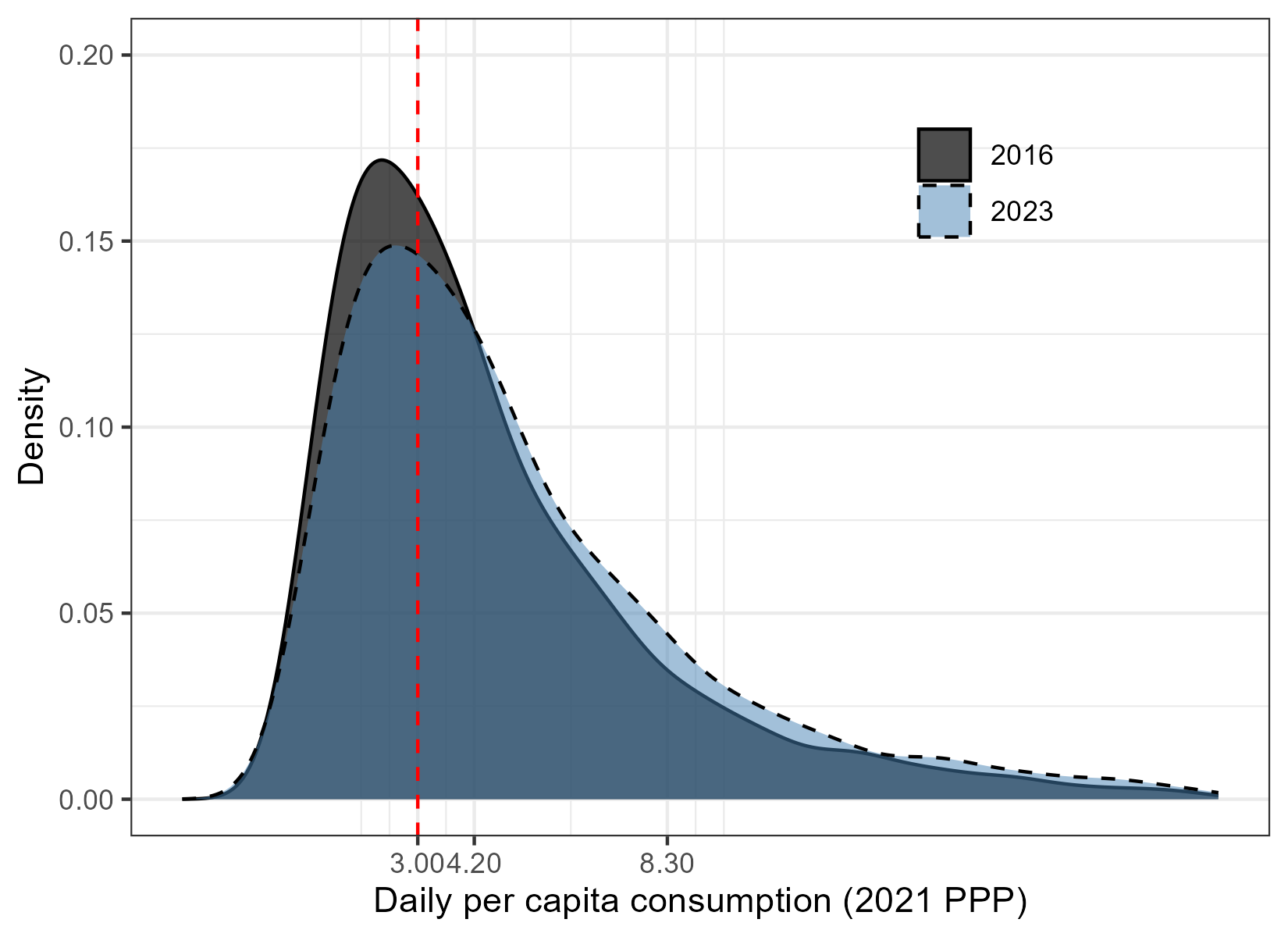
Interpolated and extrapolated values

R code
R output
Stata code
Stata output

get_stats(country = "GHA", fill_gaps = TRUE)  |> 
  filter(year >= 2016) |>
  select(country_code, year, poverty_line, headcount)

# A tibble: 9 × 4
  country_code  year poverty_line headcount
  <chr>        <dbl>        <dbl>     <dbl>
1 GHA           2016            3     0.405
2 GHA           2017            3     0.385
3 GHA           2018            3     0.375
4 GHA           2019            3     0.359
5 GHA           2020            3     0.366
6 GHA           2021            3     0.355
7 GHA           2022            3     0.348
8 GHA           2023            3     0.345
9 GHA           2024            3     0.332

pip, country(GHA) year(2016/2025) n2disp(5) fillgaps nowcasts clear

version in use 20260324_2021_01_02_PROD

first 5 observations

  +------------------------------------------------------------------------+
  | country_code   year   poverty_line   headcount     mean   welfare_type |
  |------------------------------------------------------------------------|
  |          GHA   2016           3.00      0.4046   4.9054    consumption |
  |          GHA   2017           3.00      0.3852   5.1186    consumption |
  |          GHA   2018           3.00      0.3753   5.2626    consumption |
  |          GHA   2019           3.00      0.3593   5.4244    consumption |
  |          GHA   2020           3.00      0.3655   5.3686    consumption |
  +------------------------------------------------------------------------+
Click here to display how to cite

Versioning with PIP

Access various vintages of the data with the versioning options (shown here in R).

R code
R output

get_versions()

# A tibble: 16 × 4
   version                  release_version ppp_version identity
   <chr>                    <chr>           <chr>       <chr>   
 1 20260324_2021_01_02_PROD 20260324        2021        PROD    
 2 20260324_2017_01_02_PROD 20260324        2017        PROD    
 3 20250930_2021_01_02_PROD 20250930        2021        PROD    
 4 20250930_2017_01_02_PROD 20250930        2017        PROD    
 5 20250401_2021_01_02_PROD 20250401        2021        PROD    
 6 20250401_2017_01_02_PROD 20250401        2017        PROD    
 7 20240627_2017_01_02_PROD 20240627        2017        PROD    
 8 20240627_2011_02_02_PROD 20240627        2011        PROD    
 9 20240326_2017_01_02_PROD 20240326        2017        PROD    
10 20240326_2011_02_02_PROD 20240326        2011        PROD    
11 20230919_2017_01_02_PROD 20230919        2017        PROD    
12 20230919_2011_02_02_PROD 20230919        2011        PROD    
13 20230328_2017_01_02_PROD 20230328        2017        PROD    
14 20230328_2011_02_02_PROD 20230328        2011        PROD    
15 20220909_2017_01_02_PROD 20220909        2017        PROD    
16 20220909_2011_02_02_PROD 20220909        2011        PROD

Versioning with PIP

R code
R output
Stata code
Stata output

get_stats("IND", version = "20260324_2021_01_02_PROD") |> 
  select(country_code, country_name, year, poverty_line, headcount, reporting_level, survey_acronym) |> tail(3)

# A tibble: 3 × 7
  country_code country_name  year poverty_line headcount reporting_level
  <chr>        <chr>        <dbl>        <dbl>     <dbl> <chr>          
1 IND          India         2009            3    0.346  national       
2 IND          India         2011            3    0.271  national       
3 IND          India         2022            3    0.0525 national       
# ℹ 1 more variable: survey_acronym <chr>

pip, country(IND) version(20260324_2021_01_02_PROD) clear
list country_code country_name year poverty_line headcount reporting_level survey_acronym in -3/L

first observation

  +------------------------------------------------------------------------+
  | country_code   year   poverty_line   headcount     mean   welfare_type |
  |------------------------------------------------------------------------|
  |          IND   1977           3.00      0.5970   3.1832    consumption |
  +------------------------------------------------------------------------+
Click here to display how to cite

     +------------------------------------------------------------------------+
     | count~de   count~me   year   povert~e   headco~t   report~l   survey~m |
     |------------------------------------------------------------------------|
  6. |      IND      India   2009       3.00     0.3458   national   NSS-SCH1 |
  7. |      IND      India   2011       3.00     0.2712   national   NSS-SCH2 |
  8. |      IND      India   2022       3.00     0.0525   national       HCES |
     +------------------------------------------------------------------------+

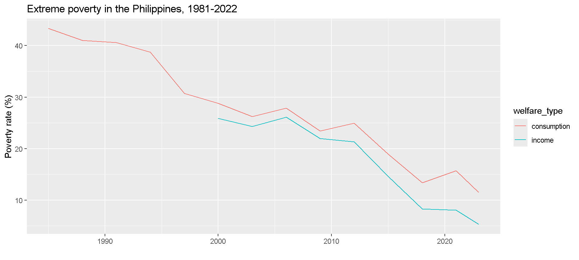
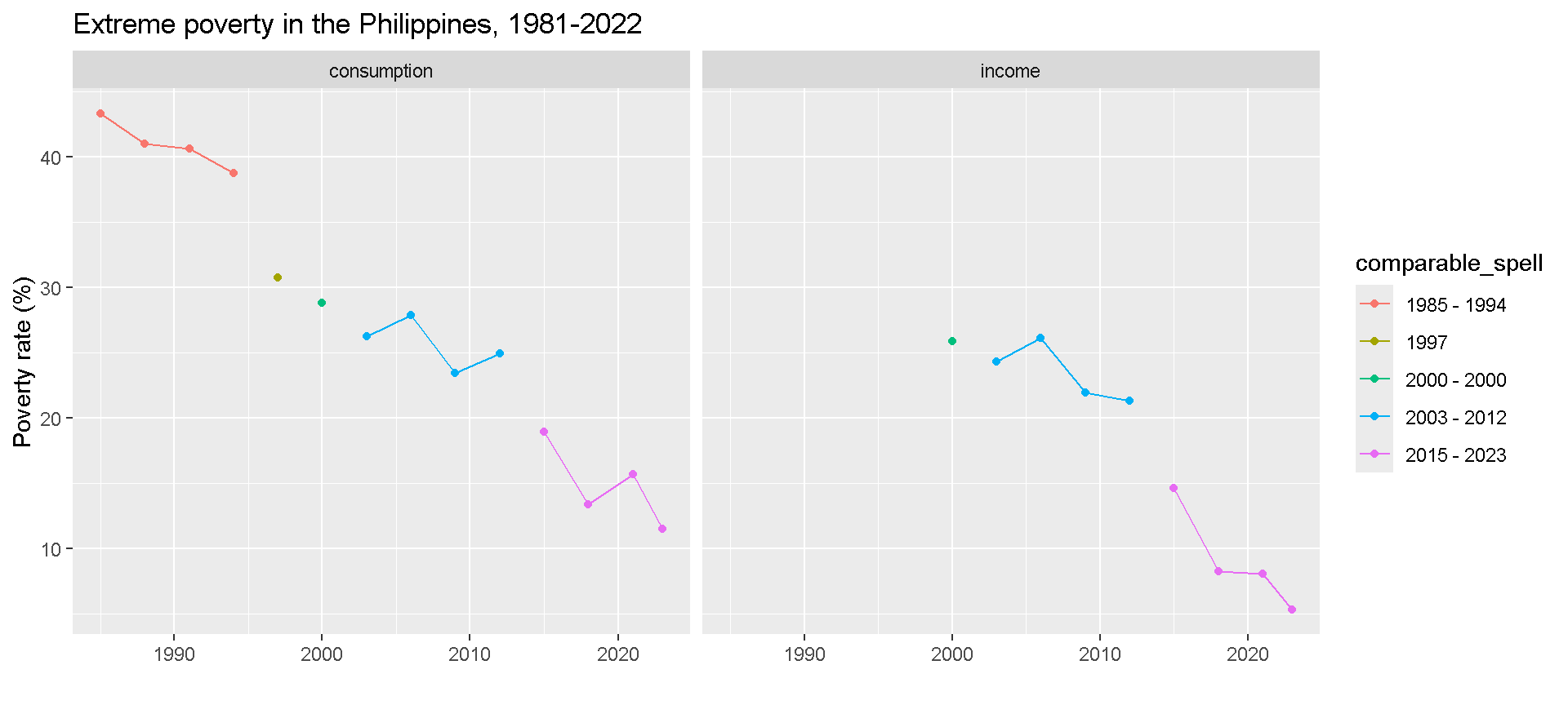
Poverty by welfare type

R code
R output
Stata code
Stata output

df <- get_stats(country = "PHL")       
gr <- ggplot(df, aes(y = 100*headcount, x = year, color = welfare_type)) +          
      geom_line() +                     
      labs(title = "Extreme poverty in the Philippines, 1981-2022",                       
           y     = "Poverty rate (%)",                          
           x     = "")
gr

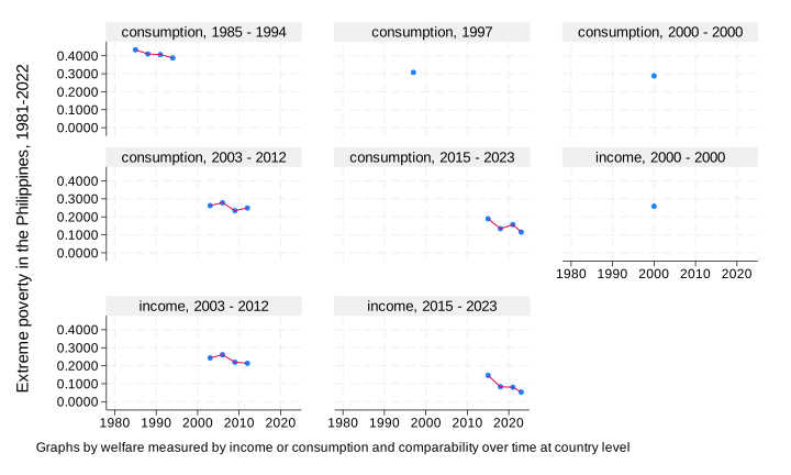
pip, country(PHL) clear
graph twoway line headcount year, by(welfare_type) xtitle("") ytitle("Extreme poverty in the Philippines, 1981-2022")
graph export "img/welfare_plot.svg", replace

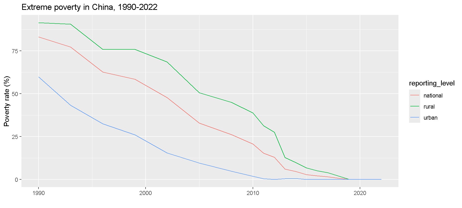
Poverty by reporting level

R code
R output
Stata code
Stata output

df <- get_stats(country = "CHN") |>
      filter(year >= 1990)
  
gr <- ggplot(df, aes(y = 100*headcount, x = year, color = reporting_level)) +
      geom_line() + 
      labs(title = "Extreme poverty in China, 1990-2022",
           y     = "Poverty rate (%)",
           x     = "")
gr

pip, country(CHN) year(1990/2022) clear
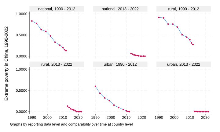
graph twoway line headcount year || scatter headcount year, by(reporting_level comparable_spell, legend(off)) xtitle("") ytitle("Extreme poverty in China, 1990-2022")
graph export "img/rep_level_plot.svg", replace

Within-country comparability

R code
R output
Stata code
Stata output

df <- get_stats(country = "CHN") |> 
      filter(reporting_level == "national" & year >= 1990) |>
      select(year, headcount, comparable_spell, welfare_type)
print(df, n = 21)

# A tibble: 20 × 4
    year headcount comparable_spell welfare_type
   <dbl>     <dbl> <chr>            <chr>       
 1  1990   0.831   1990 - 2012      consumption 
 2  1993   0.773   1990 - 2012      consumption 
 3  1996   0.626   1990 - 2012      consumption 
 4  1999   0.585   1990 - 2012      consumption 
 5  2002   0.478   1990 - 2012      consumption 
 6  2005   0.329   1990 - 2012      consumption 
 7  2008   0.261   1990 - 2012      consumption 
 8  2010   0.206   1990 - 2012      consumption 
 9  2011   0.153   1990 - 2012      consumption 
10  2012   0.129   1990 - 2012      consumption 
11  2013   0.0604  2013 - 2022      consumption 
12  2014   0.0461  2013 - 2022      consumption 
13  2015   0.0286  2013 - 2022      consumption 
14  2016   0.0209  2013 - 2022      consumption 
15  2017   0.0157  2013 - 2022      consumption 
16  2018   0.00750 2013 - 2022      consumption 
17  2019   0       2013 - 2022      consumption 
18  2020   0       2013 - 2022      consumption 
19  2021   0       2013 - 2022      consumption 
20  2022   0       2013 - 2022      consumption

keep if reporting_level=="national"
list country_name reporting_level year headcount comparable_spell welfare_type

(40 observations deleted)

     +-------------------------------------------------------------------+
     | count~me   report~l   year   headco~t   comparabl~l   welfare_~pe |
     |-------------------------------------------------------------------|
  1. |    China   national   1990     0.8311   1990 - 2012   consumption |
  2. |    China   national   1993     0.7728   1990 - 2012   consumption |
  3. |    China   national   1996     0.6262   1990 - 2012   consumption |
  4. |    China   national   1999     0.5847   1990 - 2012   consumption |
  5. |    China   national   2002     0.4779   1990 - 2012   consumption |
     |-------------------------------------------------------------------|
  6. |    China   national   2005     0.3291   1990 - 2012   consumption |
  7. |    China   national   2008     0.2606   1990 - 2012   consumption |
  8. |    China   national   2010     0.2058   1990 - 2012   consumption |
  9. |    China   national   2011     0.1529   1990 - 2012   consumption |
 10. |    China   national   2012     0.1288   1990 - 2012   consumption |
     |-------------------------------------------------------------------|
 11. |    China   national   2013     0.0604   2013 - 2022   consumption |
 12. |    China   national   2014     0.0461   2013 - 2022   consumption |
 13. |    China   national   2015     0.0286   2013 - 2022   consumption |
 14. |    China   national   2016     0.0209   2013 - 2022   consumption |
 15. |    China   national   2017     0.0157   2013 - 2022   consumption |
     |-------------------------------------------------------------------|
 16. |    China   national   2018     0.0075   2013 - 2022   consumption |
 17. |    China   national   2019     0.0000   2013 - 2022   consumption |
 18. |    China   national   2020     0.0000   2013 - 2022   consumption |
 19. |    China   national   2021     0.0000   2013 - 2022   consumption |
 20. |    China   national   2022     0.0000   2013 - 2022   consumption |
     +-------------------------------------------------------------------+

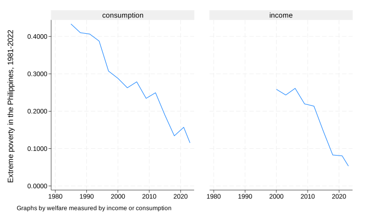
Comparability over time

R code
R output
Stata code
Stata output

df <- get_stats(country = "PHL")
  
gr <- ggplot(df, aes(y = 100*headcount, x = year, color = comparable_spell)) +
      geom_point() +
      geom_line() + 
      facet_wrap(~welfare_type) +
      labs(title = "Extreme poverty in the Philippines, 1981-2022",
           y     = "Poverty rate (%)",
           x     = "")
gr

pip, country(PHL) clear
graph twoway scatter headcount year || line headcount year, by(welfare_type comparable_spell, legend(off)) xtitle("") ytitle("Extreme poverty in the Philippines, 1981-2022")
graph export "img/welfare_plot_2.svg", replace

Data on Shared Prosperity and inequality

The World Bank recently adopted the Prosperity Gap to capture shared prosperity.
The Prosperity Gap is a average societal shortfall from a prosperity standard, currently set at $28/day in 2021 PPP. The threshold is close to the income levels of individuals living in middle income countries that is transitioning into high income status.
The data on Prosperity Gap and inequality measures are available in both the R and Stata output.

Data on Shared Prosperity and inequality

R code
R output
Stata code
Stata output

get_stats(country = "GHA") |>
  select(country_code, year, gini, pg) |>
  head(3)

# A tibble: 3 × 4
  country_code  year  gini    pg
  <chr>        <dbl> <dbl> <dbl>
1 GHA           1987 0.353  17.9
2 GHA           1988 0.360  17.5
3 GHA           1991 0.384  20.0

qui pip, clear country(GHA)
list country_code year gini pg in 1/3

     | count~de   year     gini          pg |
     |--------------------------------------|
  1. |      GHA   1987   0.3535    17.87457 |
  2. |      GHA   1988   0.3599   17.467325 |
  3. |      GHA   1991   0.3843   19.958958 |
     +--------------------------------------+

Data from LIS

R code
R output
Stata code
Stata output

get_stats() |>
  filter(grepl("LIS", survey_acronym)) |>
  group_by(country_name) |>
  summarize(obs = n()) |>
  ungroup() |> 
  arrange(desc(obs)) |>
  print(n = 29)

# A tibble: 29 × 2
   country_name      obs
   <chr>           <int>
 1 United States      62
 2 United Kingdom     54
 3 Canada             46
 4 Germany            32
 5 Israel             26
 6 Luxembourg         18
 7 Italy              17
 8 Taiwan, China      16
 9 Australia          13
10 Japan              13
11 France             12
12 Korea, Rep.        11
13 Spain              11
14 Sweden              8
15 Austria             7
16 Belgium             6
17 Ireland             6
18 Netherlands         5
19 Norway              5
20 Switzerland         5
21 Denmark             4
22 Finland             4
23 Poland              4
24 Czechia             3
25 Greece              3
26 Hungary             3
27 Romania             2
28 Slovak Republic     2
29 Slovenia            2

qui pip, clear
keep if strpos(survey_acronym,"LIS")
tab country_name

(2,184 observations deleted)

          country/economy name |      Freq.     Percent        Cum.
-------------------------------+-----------------------------------
                     Australia |         13        3.25        3.25
                       Austria |          7        1.75        5.00
                       Belgium |          6        1.50        6.50
                        Canada |         46       11.50       18.00
                       Czechia |          3        0.75       18.75
                       Denmark |          4        1.00       19.75
                       Finland |          4        1.00       20.75
                        France |         12        3.00       23.75
                       Germany |         32        8.00       31.75
                        Greece |          3        0.75       32.50
                       Hungary |          3        0.75       33.25
                       Ireland |          6        1.50       34.75
                        Israel |         26        6.50       41.25
                         Italy |         17        4.25       45.50
                         Japan |         13        3.25       48.75
                   Korea, Rep. |         11        2.75       51.50
                    Luxembourg |         18        4.50       56.00
                   Netherlands |          5        1.25       57.25
                        Norway |          5        1.25       58.50
                        Poland |          4        1.00       59.50
                       Romania |          2        0.50       60.00
               Slovak Republic |          2        0.50       60.50
                      Slovenia |          2        0.50       61.00
                         Spain |         11        2.75       63.75
                        Sweden |          8        2.00       65.75
                   Switzerland |          5        1.25       67.00
                 Taiwan, China |         16        4.00       71.00
                United Kingdom |         54       13.50       84.50
                 United States |         62       15.50      100.00
-------------------------------+-----------------------------------
                         Total |        400      100.00

Global and regional estimates

R code
R output
Stata code
Stata output

get_wb()

# A tibble: 460 × 14
   region_code region_name        year poverty_line    pop headcount poverty_gap
   <chr>       <chr>             <dbl>        <dbl>  <dbl>     <dbl>       <dbl>
 1 AFE         Eastern and Sout…  1981            3 2.38e8     0.597       0.279
 2 AFE         Eastern and Sout…  1982            3 2.46e8     0.599       0.282
 3 AFE         Eastern and Sout…  1983            3 2.54e8     0.606       0.289
 4 AFE         Eastern and Sout…  1984            3 2.61e8     0.615       0.295
 5 AFE         Eastern and Sout…  1985            3 2.69e8     0.623       0.300
 6 AFE         Eastern and Sout…  1986            3 2.78e8     0.618       0.296
 7 AFE         Eastern and Sout…  1987            3 2.86e8     0.611       0.293
 8 AFE         Eastern and Sout…  1988            3 2.94e8     0.611       0.293
 9 AFE         Eastern and Sout…  1989            3 3.03e8     0.609       0.290
10 AFE         Eastern and Sout…  1990            3 3.12e8     0.616       0.295
# ℹ 450 more rows
# ℹ 7 more variables: poverty_severity <dbl>, watts <dbl>, mean <dbl>,
#   spr <dbl>, pg <dbl>, pop_in_poverty <dbl>, estimate_type <chr>

pip wb, clear

levelsof region_code

version in use 20260324_2021_01_02_PROD

first observation

  +---------------------------------------------------------+
  | region_code   year   poverty_line   headcount      mean |
  |---------------------------------------------------------|
  |         WLD   1981           3.00      0.4711   11.8277 |
  +---------------------------------------------------------+
Click here to display how to cite

`"EAS"' `"ECS"' `"LCN"' `"MEA"' `"NAC"' `"SAS"' `"SSF"' `"WLD"'

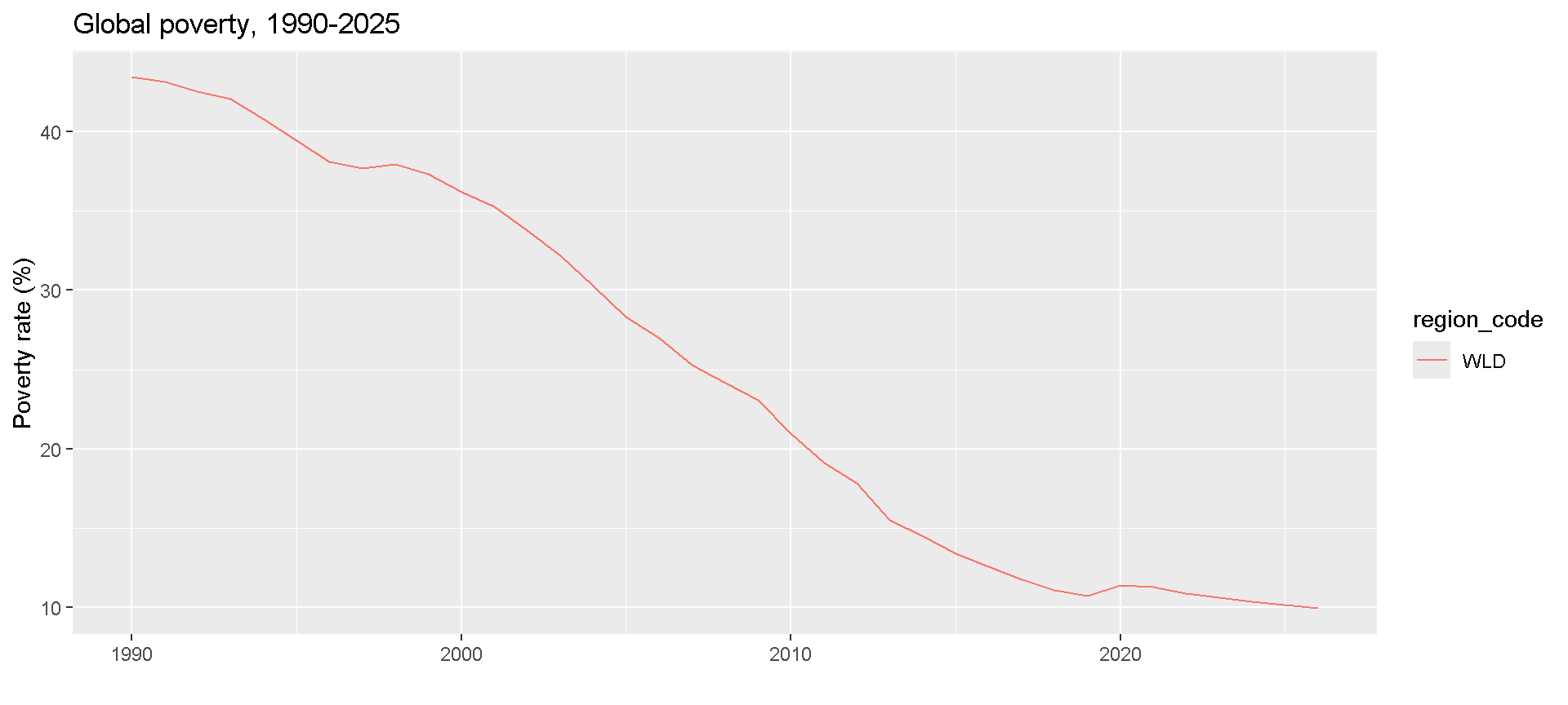
Global poverty, 1990-2022

R code
R output
Stata code
Stata output

df <- get_wb() |>
      filter(year >= 1990, region_code %in% c("WLD","EAP","SSA"))

gr <- ggplot(df, aes(x = year, y = 100*headcount, color = region_code)) +
  geom_line() +
  labs(title = "Global poverty, 1990-2025",
       y     = "Poverty rate (%)",
       x     = "") 
gr

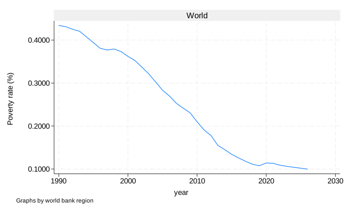
keep if year>=1990 & inlist(region_code,"WLD","EAP","SSA")
graph twoway line headcount year, by(region_name) ytitle("Poverty rate (%)") ///
ylab(,angle(horizontal))

graph export "img/pov_90_22.svg", replace

Many more functions

R code
R output
Stata code
Stata output

ls("package:pipr")

 [1] "call_aux"                    "change_grouped_stats_to_csv"
 [3] "check_api"                   "datt_rural"                 
 [5] "datt_urban"                  "delete_cache"               
 [7] "display_aux"                 "get_agg"                    
 [9] "get_aux"                     "get_cache_info"             
[11] "get_cp"                      "get_cp_ki"                  
[13] "get_gd"                      "get_pip_info"               
[15] "get_stats"                   "get_versions"               
[17] "get_wb"

pip tables

version in use 20260324_2021_01_02_PROD
Auxiliary tables available for :
     01 | aux_versions
     02 | countries
     03 | country_coverage
     04 | country_list
     05 | cpi
     06 | decomposition
     07 | dictionary
     08 | framework
     09 | gdp
     10 | incgrp_coverage
     11 | indicators
     12 | interpolated_means
     13 | metaregion
     14 | missing_data
     15 | pce
     16 | pg_lnp
     17 | pg_svy
     18 | pop
     19 | pop_region
     20 | poverty_lines
     21 | ppp
     22 | region_coverage
     23 | regions
     24 | spr_lnp
     25 | spr_svy
     26 | survey_means

4. Exercises

Exercise 1

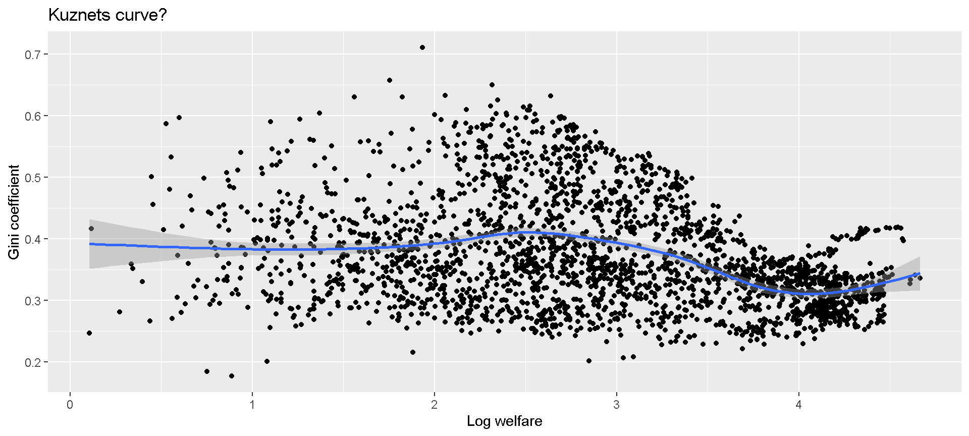
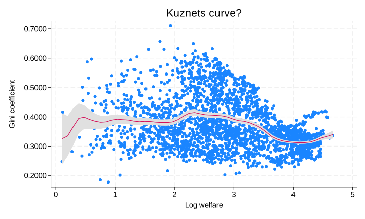
Explore whether Kuznets’ inverse-U hypothesis holds with data in PIP

Plot the relationship between an inequality metric and log mean welfare
Regress an inequality metric on a 2nd order polynomial of log mean welfare

Results

R code
R regression
R graph
Stata code
Stata regression
Stata graph

# Kuznets curve? 
df <- get_stats()   
gr <- ggplot(df, aes(x = log(mean), y = gini)) +   
      geom_point() +   
      geom_smooth() +   
      labs(title = "Kuznets curve?",
           y     = "Gini coefficient",
           x     = "Log welfare")   
m <- lm(gini ~ log(mean) + I(log(mean)^2), data = df)
summary(m)


Call:
lm(formula = gini ~ log(mean) + I(log(mean)^2), data = df)

Residuals:
      Min        1Q    Median        3Q       Max 
-0.200072 -0.052464 -0.009036  0.045227  0.307608 

Coefficients:
                Estimate Std. Error t value Pr(>|t|)    
(Intercept)     0.322785   0.011533  27.989   <2e-16 ***
log(mean)       0.078876   0.008691   9.075   <2e-16 ***
I(log(mean)^2) -0.019365   0.001542 -12.557   <2e-16 ***
---
Signif. codes:  0 '***' 0.001 '**' 0.01 '*' 0.05 '.' 0.1 ' ' 1

Residual standard error: 0.07955 on 2581 degrees of freedom
Multiple R-squared:  0.1495,    Adjusted R-squared:  0.1488 
F-statistic: 226.8 on 2 and 2581 DF,  p-value: < 2.2e-16

pip, clear

gen logmean = log(mean)
gen logmean2 = log(mean)^2

reg gini logmean logmean2

graph twoway scatter gini logmean || ///
lpolyci gini logmean, ///
title("Kuznets curve?") ///
xtitle("Log welfare") ///
ytitle("Gini coefficient") ///
legend(off)

graph export "img/ex_1_plot.svg", replace

      Source |       SS           df       MS      Number of obs   =     2,584
-------------+----------------------------------   F(2, 2581)      =    226.80
       Model |  2.87042776         2  1.43521388   Prob > F        =    0.0000
    Residual |  16.3328866     2,581  .006328123   R-squared       =    0.1495
-------------+----------------------------------   Adj R-squared   =    0.1488
       Total |  19.2033144     2,583    .0074345   Root MSE        =    .07955

------------------------------------------------------------------------------
        gini | Coefficient  Std. err.      t    P>|t|     [95% conf. interval]
-------------+----------------------------------------------------------------
     logmean |   .0788755   .0086913     9.08   0.000     .0618329    .0959181
    logmean2 |  -.0193649   .0015422   -12.56   0.000    -.0223889   -.0163409
       _cons |   .3227849   .0115326    27.99   0.000     .3001707    .3453991
------------------------------------------------------------------------------

Exercise 2

COVID-19 impact on poverty and inequality

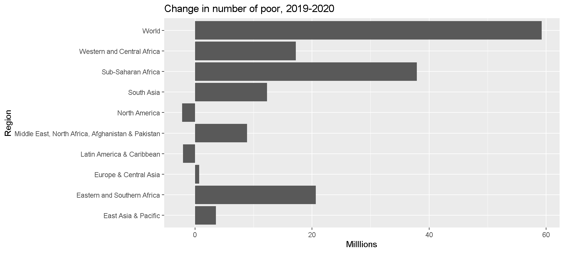
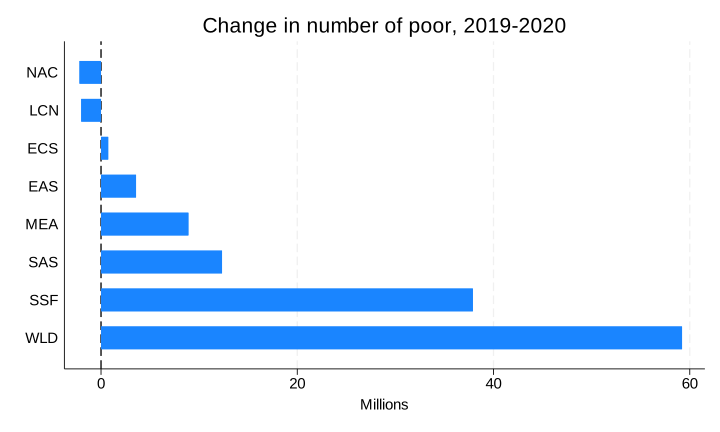
Calculate and plot the change in millions of extreme poor by region from 2019 to 2020
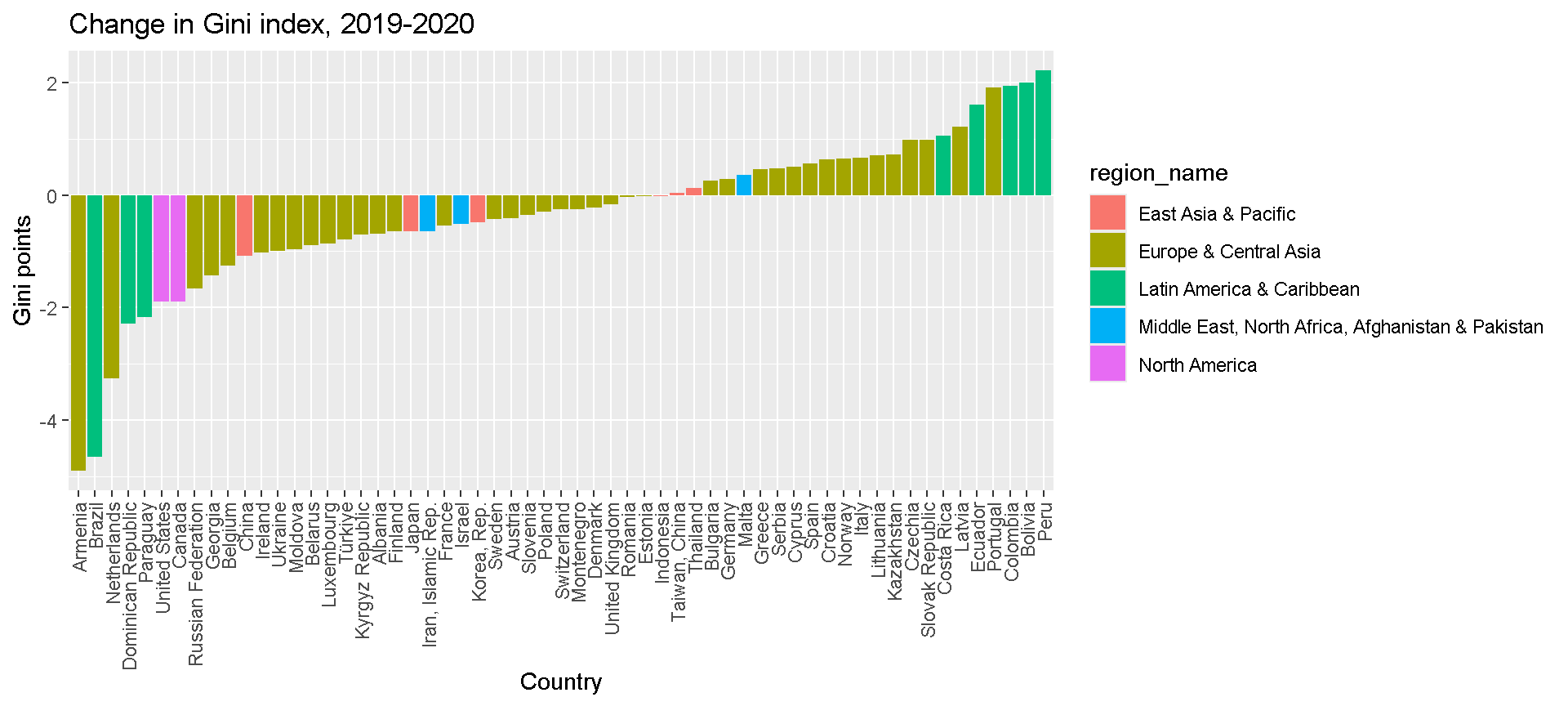
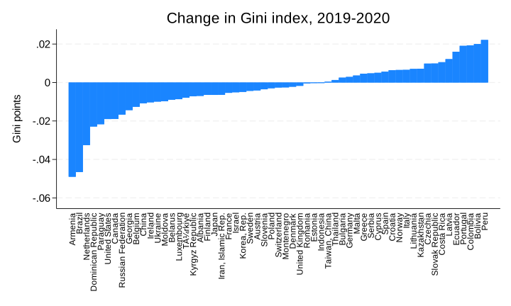
(Difficult) Calculate and plot the changes in Gini observed from 2019 to 2020 for countries with comparable data during these two years

Results (part 1)

R code
R output
Stata code
Stata output

# Change in number of poor, 2019-2020
df <- get_wb() |> filter(year == 2019 | year == 2020) |>
      group_by(region_code) |>
      mutate(changeinpoor = pop_in_poverty - lag(pop_in_poverty)) |>
      filter(!is.na(changeinpoor))

gr <- ggplot(df, aes(y = region_name, x = changeinpoor/10^6)) +
  geom_bar(stat = "identity") +
  labs(title = "Change in number of poor, 2019-2020", x = "Milllions", y = "Region") 
gr

* Without the nowcast option, data will only be presented for regions with sufficient data coverage

pip wb, nowcasts clear
keep if year==2019 | year==2020
bysort region_code (year): gen changeinpoor = (pop_in_poverty-pop_in_poverty[_n-1])/10^6
keep if year==2020

graph hbar changeinpoor, over(region_code, sort(changeinpoor)) ytitle("Millions") title("Change in number of poor, 2019-2020") yline(0)

graph export "img/ex_2a_plot.svg", replace

Results (part 2)

R code
R output
Stata code
Stata output

# Change in Gini, 2019-2020?
df <- get_stats() |> 
      filter(year == 2019 | year == 2020) |>
      filter(reporting_level == "national") |>
      group_by(country_code, welfare_type, comparable_spell) |>
      # Only keeps countries with comparable estimates in 2019 and 2020
      filter(n() == 2) |>
      mutate(ginichange = gini - lag(gini)) |>
      filter(year == 2020) |>
      ungroup() |>
      # If countries have both income and consumption estimates, use only the latter
      group_by(country_code) |>
      filter(n() == 1 | welfare_type == "consumption") |>
      ungroup()

gr <- ggplot(df[df$country_code != "XKX",], aes(x = reorder(country_name, +ginichange), y = ginichange*100, fill = region_name)) +
  geom_bar(stat = "identity") +
  labs(title = "Change in Gini index, 2019-2020", y = "Gini points", x = "Country") +
  theme(axis.text.x = element_text(angle = 90, vjust = 0.5, hjust = 1))
gr

pip, year(2019/2020) coverage(national)

*Only keep countries with comparable estimates in 2019 and 2020:

bysort country_code welfare_type comparable_spell: keep if _N==2
bysort country_code welfare_type comparable_spell (year): gen ginichange = gini-gini[_n-1]
keep if year==2020

*If countries have both income and consumption estimates, use only the latter:

bysort country_code: keep if _N==1 |  welfare_type==1

*Something strange is going on with Kosovo:

drop if country_code=="XKX"

*Draw graph

graph bar ginichange,  over(country_name, sort(ginichange)  gap(0) lab(angle(90) labsize(small)))   ///
title("Change in Gini index, 2019-2020") ytitle("Gini points") 

graph export "img/ex_2b_plot.svg", replace

5. Additional resources

Methodological handbook: Describes all methodological details behind the estimates
Poverty & Inequality Briefs: 2-page summary of poverty and inequality in almost every developing country
Survey percentiles: 100 percentiles of each country-year survey distribution
Lined-up percentiles distribution: 1000 points on the global distribution
Accessing some of the microdata online
More data and indicators through the user interface
API access

Acknowledgment

The findings, interpretations, and conclusions expressed in this presentation are entirely those of the author. They do not necessarily represent the views of the World Bank and its affiliated organizations, or those of the Executive Directors of the World Banks or the governments they represent.

The authors gratefully acknowledge financial support from the UK government through the Data and Evidence for Tackling Extreme Poverty (DEEP) Research Programme.

Thank you for listening!

For further details please contact:

Diana C. Garcia Rojas: dgarciarojas@worldbank.org
Zander Prinsloo: zprinsloo@worldbank.org
Rossana Tatulli: rtatulli@worldbank.org
Nishant Yonzan: nyonzan@worldbank.org

Poverty and Inequality Platform (PIP): An introduction using R and Stata

Outline

1. Introduction

Poverty data at the World Bank

The Poverty and Inequality Platform (PIP)

PIP motivation

PIP: Transparency

PIP: Transparency

Data release notes and other publications

Data on inequality

Welfare measure reported in PIP

Acquiring Household Data

Constructing Welfare Aggregates

Adjusting Welfare Aggregates

Calculating survey estimates

Calculating regional aggregates

2. Accessing PIP through the user interface

3. Accessing PIP in R and Stata

Installation

Two main functions

Country-level estimates

Variables

Auxiliary data

Ghanaian survey estimates

Ghanaian survey estimates

Ghanaian survey estimates with 2017 PPP

Different poverty line

Multiple poverty lines

Estimates across selected countries

Extrapolation for Ghana from 2016 to most recent year

Interpolated and extrapolated values

Versioning with PIP

Versioning with PIP

Poverty by welfare type

Poverty by reporting level

Within-country comparability

Comparability over time

Data on Shared Prosperity and inequality

Data on Shared Prosperity and inequality

Data from LIS

Global and regional estimates

Global poverty, 1990-2022

Many more functions

4. Exercises

Exercise 1

Results

Exercise 2

Results (part 1)

Results (part 2)

5. Additional resources

Acknowledgment

Thank you for listening!

Poverty and Inequality Platform (PIP):
An introduction using R and Stata